Quantifying NHL Shooting Talent: A Data Driven Approach
Yes, we can do better than just the Rocket Richard Trophy.


It’s no secret that today’s NHL has undergone many transformations on both the business side and the hockey side to arrive at its current state. Competing with the three other sports leagues that make up the “big four” in North America has been an omnipresent challenge for the NHL (outside of Canada), and as a result I believe the NHL has often been behind other leagues when it comes to innovation.
One area where the NHL has had to play catch up to the other sports leagues is in the use of analytics, a broad term that can be understood as the leveraging of advanced math and statistical methods to unlock more ways of evaluating teams and players. While analytics are often subjective (as I’ve written about previously here), that does not mean they are necessarily less informative than traditional “eye test” statistics.
I would liken analytics to a tool such as a telescope - we can learn about celestial bodies by looking up at the sky with our eyes and making reference to size, brightness, etc. - but it’s not until we use a telescope that we gain deeper understanding about these objects. Since we don’t have physical access to the stars and planets, information gleaned from the telescope could be open to some interpretation. Regardless, we still get a much deeper look at what’s happening whether in the cosmos or on the rink.
The NHL, to its credit, has done a decent job of open-sourcing its game data back to the 2007-08 season which has no doubt contributed to the popularity of hockey analytics. Throughout the rest of this article I’m going to discuss a machine learning project I’ve been working on that attempts to quantify each NHL player’s “shooting talent”.
Objective
While there could be some disagreement, there’s plenty of reason to believe that hockey is the sport that is most characterized by luck. What I mean is that compared to other sports, hockey is the most likely to have factors outside of what the players can control determine the outcome of games. As a result, it is sometimes the case that the better playing team in a game does not emerge victorious.
One piece of evidence I often cite for this is the much higher rate of upsets in best-of-7 NHL playoff series compared to the NBA, where the higher seeded team wins 80% of playoff rounds with the same best-of-7 format. It may be another reason why hockey was late to the analytics party, although it also speaks to the importance of analytical solutions to make the most of what can be controlled.
One of the main weaknesses of the public expected goal models is that they have a built-in presupposition that every player is of equal (average) shooting ability and that every goaltender is also equal. It doesn’t take a hardcore hockey fan to recognize that this is probably not a realistic assumption. MoneyPuck has attempted to rectify this with their “shooting talent expected goals” metric, which uses a Bayesian approach to measure shooting talent and then calibrates the expected goal value based on who shot the puck.
A less reasonable proxy for shooting talent is raw shooting percentage (number of goals scored divided by number of shots on goal). It does not account for any factors other than the number of shots and goals, and we’ve already established that chance is very much a factor in hockey. So how can we isolate a player’s true impact on the goals they score from the randomness and other circumstances that lead to a puck entering the opponent’s net?
While we can never truly account for all randomness (by definition), there are other measurable variables that can be isolated when it comes to goal scoring in the NHL. Many of these variables can be obtained directly or indirectly from the NHL’s public data, which is what I used for this project.
My approach was largely inspired by Evolving Hockey’s Regularized Adjusted Plus-Minus (RAPM), a data-driven method for isolating individual hockey players’ and teams’ impact on multiple offensive and defensive metrics, including goals for and against. If you’re at all interested in this they have written a detailed breakdown of the subject. The idea of a quantifiable shooting talent is an extension of the aforementioned shooting talent expected goals from MoneyPuck. By combining these two concepts my goal was to introduce a useful metric for player evaluation.
Methodology
I began by gathering all shot data from every NHL game during the 2023-24 regular season (the most recent full season), excluding blocked shots, penalty shots, shootouts, and shots taken while the opposing goalie was substituted for an extra skater (i.e., empty nets). Only shots taken from the offensive/attacking zone are included in the analysis.
Further filtering was done to exclude shots by players that did not meet the minimum shot attempt threshold (calculated as the 20th percentile of shot attempts per player, which was 25 across the whole season). The remaining dataset contained details about all 108,049 offensive zone shot attempts in the 2023-24 regular season that were either goals, stopped by the opposing goalie, or missed the net - and taken by players who registered at least 25 shot attempts during that season.
Here is a list of predictor variables that went into the model:
Distance from net (feet)
Angle from net (degrees)
Shot Type (wrist, slap, backhand, etc.)
Home/Away
Was shot a rebound?
Score situation (trailing, tied, leading)
Strength situation (power play, even strength, short-handed)
Shooting player
Opposing goalie
Model Building (non-technical readers may skip this section)
A bit of feature engineering had to be done to obtain some of these variables. The NHL data contains locations of each shot as (x, y) coordinates, so knowing the rink dimensions I then calculated the distance and angle from the net with basic trigonometry. A shot is classified as coming off a rebound if there was another shot taken within the prior 3 second window. The strength situation is determined by number of skaters on the ice. So while technically a goalie substituted for an extra skater would officially be considered even strength (assuming neither team has a penalty), in this case I am classifying it as a power play for the team with an extra skater.
All variables except distance and angle are categorical, meaning each observation (shot) falls into one of several categories for that particular variable (i.e., the score is either tied, trailing, or leading from the shooting player’s perspective). To make all features numerical, each categorical variable is transformed to a one-hot encoding (every category becomes its own variable indicated by a 1 or 0, image below for reference). The target variable is simply whether or not a goal was scored. Because there are just two possible outcomes (goal=1, not a goal=0), this is a binary classification problem.

The dataset was unbalanced since only 7% of shot attempts it contained were goals. Fortunately, this is something we can automatically adjust for in the model’s algorithm (thank you, Python). I chose the logistic regression model for the following reasons:
It is specifically intended for binary classification tasks.
It is ideal when the goal of the model is explanatory (as opposed to predictive). Put another way, regression assigns a coefficient to each predictor variable which can be interpreted as the variable’s isolated effect on the target.
Since each player is a variable in the model, we can obtain a number corresponding to their shooting ability (technically their impact on the probability of a shot being a goal with all other variables held constant).
The output of a logistic regression model is always between 0 and 1, and thus can be understood as a probability. In this case, it’s the probability that a given shot is a goal. So we’ve effectively built an expected goal model, except not for the purpose of predicting goals on future shots. That said, it still matters that the model has predictive power as a proxy for reliability. To measure this, I used a standard 80-20 train-test split on the dataset. The model is trained on 80% of the shots, then tested for accuracy with the remaining 20%. The chart below shows how the model performed on unseen data.
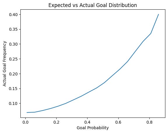
As we would hope, the actual occurrence of goals becomes more frequent as the model-generated probability increases. As such, the model is reliable (enough) to begin looking at the effect of predictor variables.
Results
After re-running the model on the entire dataset, we can now look at the coefficients. Since each player is a predictor variable, their resulting coefficient represents their shooting talent within the timeframe of the dataset (in this case, the 2023-24 regular season). A positive coefficient means above average shooting talent and negative means below average. Theoretically the average should be exactly 0 - the player has no positive or negative effect on the probability of the shot being a goal.
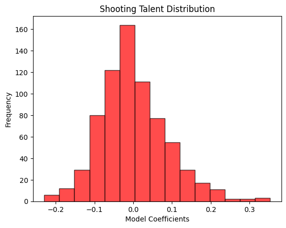
The shooting talent scores follow a Gaussian (normal) distribution, therefore we can use z-scores as a more interpretable value for shooting talent (this is also how RAPM values are assigned by Evolving Hockey). Switching to z-scores of the coefficients as our shooting talent measure, here’s how they compare to the number of shot attempts taken when viewed as a scatter plot.
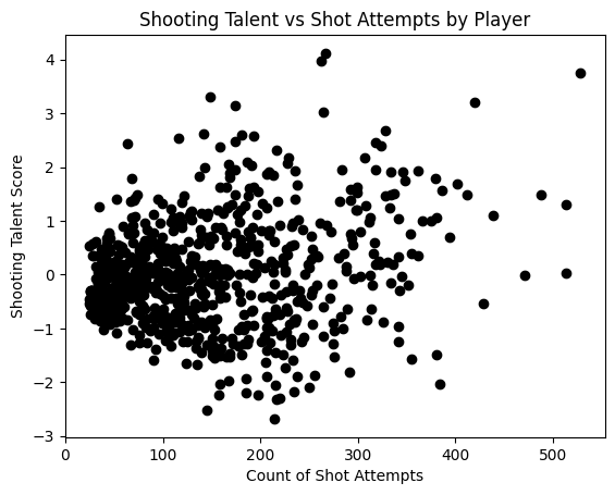
You can see that the variance of shooting talent is lower and clusters around the mean for players with lower shot counts. This was a deliberate choice resulting from the use of regularization. Since fewer shots imply less information about a player’s shooting ability, it’s reasonable to “rein in” the coefficients assigned to these players by the model. As shot attempts gradually increase, the law of large numbers kicks in and we get a more accurate estimate of a player’s shooting talent. Regularization essentially corrects for the uncertainty caused by smaller samples.
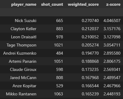
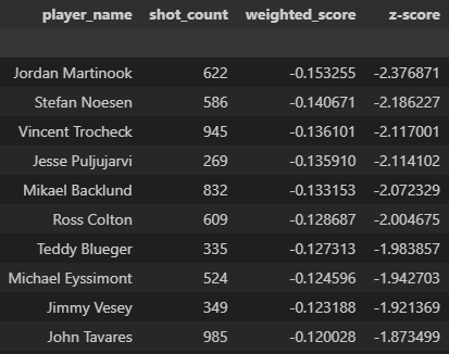
Finally, here are the top 10 and bottom 10 shooters in the NHL based on a 3-year average shooting talent score, weighted by their shot attempts. Note that I simply ran the same procedure on the 2022-2023 season and 2024-2025 season (as of March 18) and calculated the weighted average score for each player that played in all of the last 3 seasons.
Strengths, Weaknesses, and Conclusion
I think the main advantage of this model for addressing shooting ability is that it isolates a player’s impact from so many other variables that contribute to goals being scored. The amount of goals a player scores is arguably the biggest determinant (along with points) of how much they are going to get paid. A hot streak for a player over half of a season can quite literally yield millions more dollars on their next contract.
In a hard salary cap system like the NHL has in place, teams are desperate for any information that could lessen their chance of dishing out regrettable contracts while at the same time raising the possibility of finding hidden gems at a bargain. Stats like shooting talent are critical for evaluating if a player is worth the investment that his goal total commands or if he was just temporarily smiled upon by Lady Fortuna. On the other hand, a player’s shooting talent is correlated with their number of goals, so specific snapshots in time may result in much different scores for the same player.
Another downside of the model is that it does not account for a player’s shooting talent over their entire career. Theoretically this could be done, but it would require a lot more data curation. Since there is plenty of variance in how many games each player has played, there’s also the argument that era could be a factor (goal-scoring is up substantially from what it was ten years ago). With that in mind, and with the recency effect involved in player valuations, having a fixed window of no more than a few seasons may actually be more practical.
I’m by no means an expert of hockey or machine learning, but I wanted to get something written down about an experiment that I’ve enjoyed spending time on. It also aided my own understanding of the topics and even inspired some project modifications along the way. I’ll sign off with a quote from the movie Moneyball (2011) that succinctly captures the essence of analytics in professional sports:
Billy, this is Chad Bradford. He's a relief pitcher. He is one of the most undervalued players in baseball. His defect is that he throws funny. Nobody in the big leagues cares about him, because he looks funny. This guy could be not just the best pitcher in our bullpen, but one of the most effective relief pitchers in all of baseball. This guy should cost $3 million a year. We can get him for $237,000.